Visualizing your network is one of the fundamental steps in network analysis. As soon as you import your matrix, you can display the network in a graph. Sometimes, like with ORA, you need specifically to tell the software application to visualize the network.
Nevertheless, before dealing with the graph and the visual aspect of the network, it is useful to dive into how you build your matrix, because this decides the type of network you build and, consequently, the graph that will be generated. In the second article of this series, I have shown some matrices and discussed how you might choose what to include in your database and in your analysis. Now it is time to explore how you build your matrix.
The two-mode matrix
In network analysis, especially when undirected networks are involved, it helps to think in pairs: how each element of a group is linked (or not) to each element in another group. These pairs are technically called “dyads”. Since the data is usually in the form of a spreadsheet, it helps to visualize what follows as if we are looking at a spreadsheet in e.g. Microsoft Excel.
Even in one-mode networks, it makes it easier to think of two identical groups, especially when you are just starting out with network analysis. What each dyad shares is called a similarity. In a matrix, each cell corresponds to a dyad, composed of the element of the corresponding row and the element of the corresponding column. The cell shows if the dyad has similarities, and how many.
In a two-mode network, you examine two groups of different elements. In the matrix, each element of the first group is in a row, while each element of the second group is in a column. What is in each cell depends on the type of network you have.
If the network is binary, each cell has either a 0 (when the corresponding dyad has no similarities) or a 1 (if it does). There are also other ways to indicate this: for example, using an empty cell instead of a 0 and a “X” instead of a 1.
If the network is weighted, then the cell reports the number of similarities, i.e. how much they share, instead of just a 1; if there is no similarity, the cell is either empty or reports a 0. In short, in these types of matrices you analyse if and how each pair of elements in the rows is linked, based on each element in the column.
Therefore, the graph representing the network shows how the elements of the rows are connected to the ones in the column, as well as how the elements in the rows are connected among themselves, based on how many of the elements in the columns they share.
For example, in my own research, I made use of a two-mode matrix that showed a site in each row and a type of object in each column. As I explained in a previous article, this matrix was originally weighted. Each cell reported the number of contexts, whenever I had the information, in which each object was found at each site; if the number of contexts was unknown, the cell reported just a 1.
However, to avoid biases, I binarized the matrix when analysing it in ORA, showing only the presence or absence of each type of object at each site: a 0 or a 1, in other words. The resulting graph displayed not only how each site was connected to each type of object (and therefore what types were found at each site), but also how each site was connected to another, on the basis of the types found at both sites.
The one-mode matrix
In a one-mode network, you examine only the links between dyads, namely pairs of elements, of the same group. In the matrix, the rows and the columns report the same elements. Each pair or dyad thus appears twice, but inverted: first, one of the two elements will be in the row, and the other in the column, then they will switch around, with the second element in the row and the first element in the column: it becomes clearer if you look at pictures 3 and 4.
Again, what you have in the cell depends on the type of network you build. In a binary network, you have a 0 (or an empty cell) if a dyad in the group does not have any similarity, while you have a 1 (or an “X”) if the dyad shares something. In a weighted network, each cell reports how many features each dyad in the group share, and either 0 or an empty cell if they have nothing in common.
For example, in my research, the one-mode matrix reported a site in each row and in each column. Each cell stated how many similar types of objects were shared between the site of the corresponding row and the site of the corresponding column. The resulting graph showed how each site was connected to another, based on the number of types of objects shared.
Warning: with one-mode networks, beware of self-loops. If you observe the matrix, you notice that there are cells where the dyad is made of the same elements: for example, in figures 3 and 4 the site is the same. In this case, the element is connecting to itself.
It is usually better to delete self-loops, to have a clearer graph and avoid biases in the mathematical algorithms that examine the role of the elements in the network, because these algorithms also take self-loops into account. Of course, if your analysis requires it, you should keep the self-loops and give them the appropriate value derived from your data.
Should you need to delete them, you can either do that already in your matrix, with a 0 or empty cell whenever you see a self-loop (i.e. twice the exact same element), or you can easily ask the software application to do it for you, for example after importing the matrix. When you delete self-loops, you will notice that your matrix has a diagonal of cells that are empty (or display 0).
Undirected and directed networks
As I have mentioned in a previous article, networks can also be directed. In that case, the rows and columns of the matrix are the same as described for the one-mode networks. What is reported in the cells also works as already described.
However, there is an important difference. In an undirected network, each element in a dyad is considered to initiate the sharing, in a balanced and reciprocal relationship. This means that if, for example, I find that two sites share eight types of objects, I do not assume that these objects were brought from one of the two sites to the other.
Instead, I assume that both sites were the origins of sharing. As explained in the third article of this series, this is necessary when the data available does not allow you to know the place of origin of an object. This implies that a matrix for an undirected one-mode network has the same sequence of values in the rows and in the columns, and that the cell connecting each dyad will contain the same value, no matter which element of the dyad is in the row and which one is in the columns; it is like they mirror each other.
In a directed network, the link has an origin and a destination, it moves from one element of the dyad, the sender, to the other, the receiver. Hence, the relationship becomes unbalanced and has a gravity towards the receiver. As far as the matrix is concerned, that means that the rows and the columns do not mirror each other anymore. To have a clearer idea of the relationships between the elements of a directed network, especially in the graphs, it helps to think not in dyads, but in triads, namely in groups of three elements.
The cell connecting each dyad states a different value, depending on which element of the dyad is in the row and which one is in the columns. Think that the element in the row is considered the origin of the link, while the element in the column is considered the receiver, and that the cell tells if and how much the element in the row sends to the element in the column.
For example, if I focus on a pair of sites, where one of the two sends a number objects to another, when the site sending is in the row and the site receiving is in the column, the cell will show that number. Conversely, when the site receiving is the row and the site sending is in the column, my cell will show 0, because this site is not sending anything.
Of course, it can happen that both sites send something to each other. In that case, the cell will report how much the site in the row is sending to the other one. Note also that the examples just made imply a weighted network, with amounts and not simply presence/absence.
However, a directed network can be also binary, based on presence/absence. In that case, each cell will simply display if the element in the row is sending something to the element in the column; if both elements are sending something to each other, the result will simply be a reciprocal relationship.
Conclusions
In this article, I have explained a few basic things on how to “weave” your web; in other words, how to prepare your network so that it is ready to be rendered as a graph. Of course, there is always more that you can do, and how you proceed always depends on your data and on the goal of your research.
In the next article, I will show how you can work on the graph and modify it, to represent your results in an informative way.
Gallery
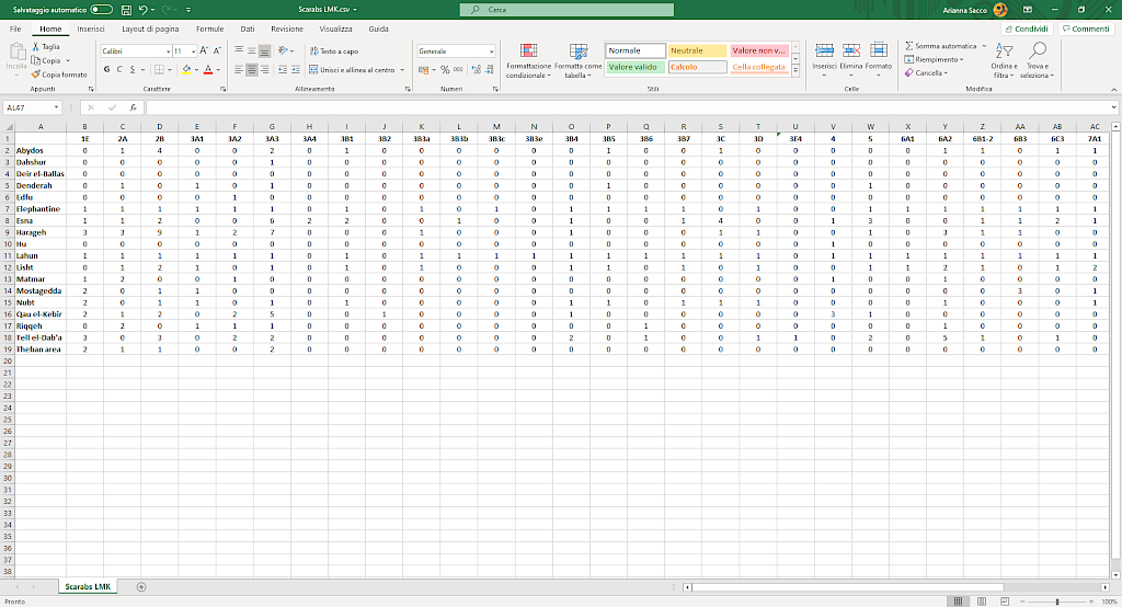
Image 1
Matrix for a two-mode network, weighted and undirected.
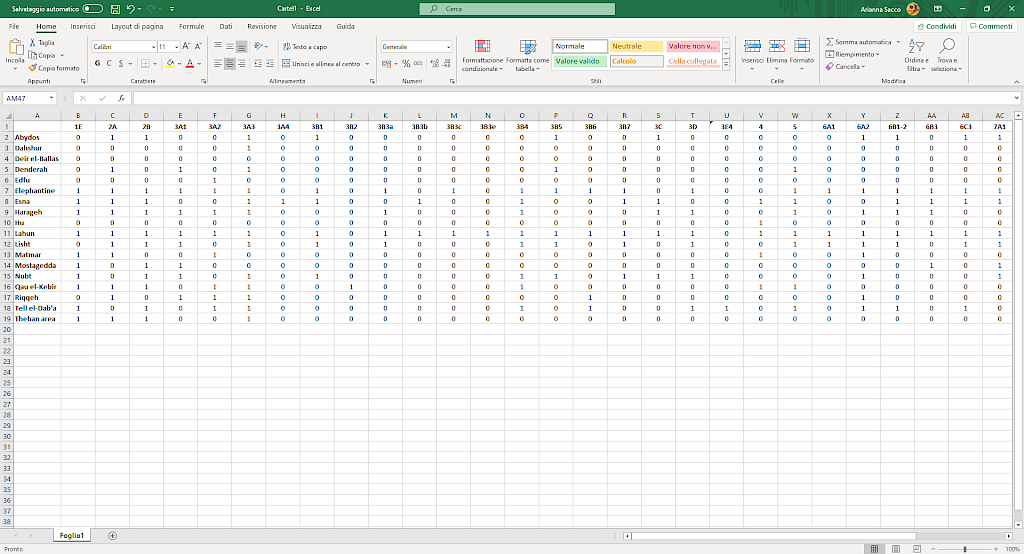
Image 2
Matrix for a two-mode network, binary and undirected.
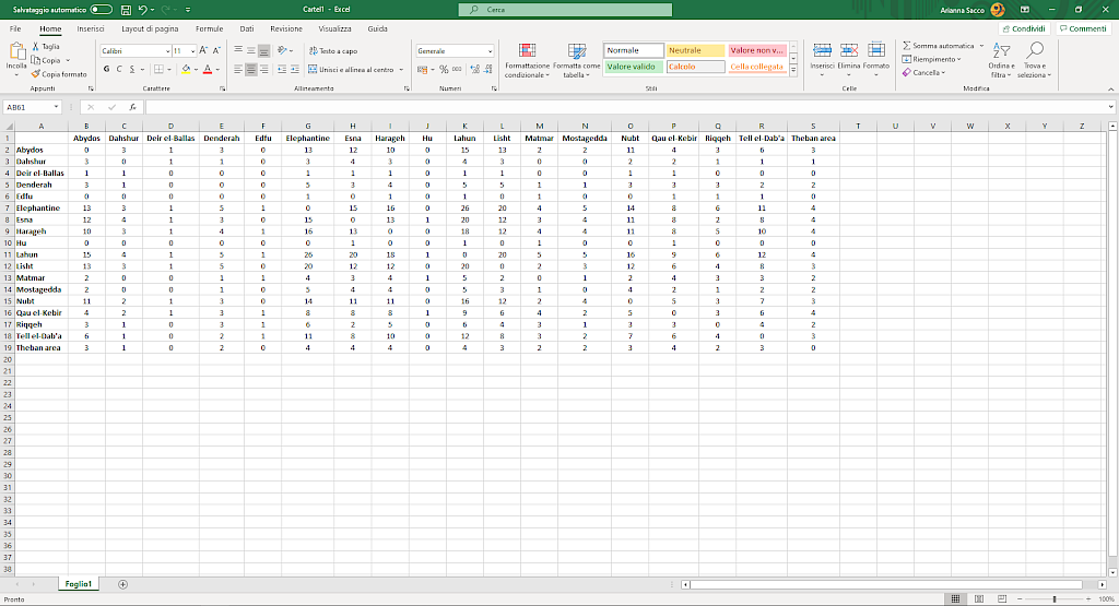
Image 3
Matrix for a one-mode network, weighted and undirected.
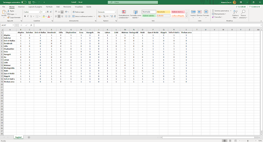
Image 4
Matrix for a one-mode network, binary and undirected.

Image 5
Matrix for a one-mode network, weighted and directed.
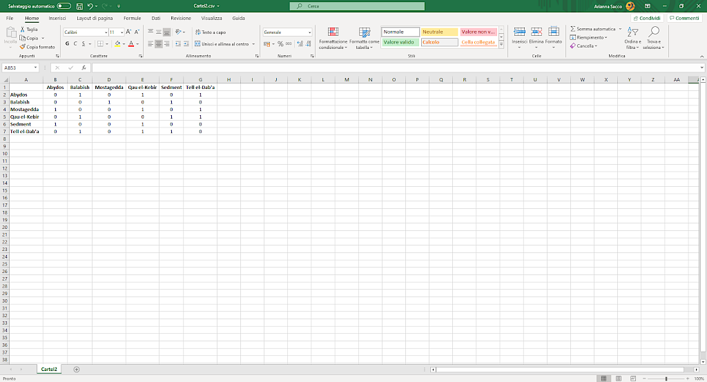
Image 6
Matrix for a one-mode network, binary and directed.
